MANOVA calculator with calculation steps, Wilks' Lambda, Pillai's Trace, Hotelling-Lawley Trace, Roy's Maximum Root.
It is followed by a Univariate ANOVA or multiple comparisons MANOVA, Box’s M test, Mahalanobis Distance test, and SW test.
Cells contain the dependent value (Y) of several subjects, and their order is important. For example, in any row, the second value of Y-1 is the same subject as the second value of Y-2. The data in each cell should be separated by Enter or , (comma).
The tool ignores empty cells or non-numeric cells.
You may copy the data from Excel, Google sheets or any tool that separate the data with Tab and Line Feed. Copy the data, one block of consecutive columns includes the header, and paste. Click to see example:
Empty cells or non-numeric cells will be ignored
How to do with R?
One-way MANOVA determines whether there is a significant difference between the averages of two or more independent groups.
An analysis of variance (ANOVA) is a special case of a multivariate analysis of variance (MANOVA)
As opposed to one-way ANOVA, where one dependent variable (Y) is assigned to each subject, MANOVA has several dependent variables (Y1, Y2, . Yp). Using the MANOVA test provided more power than running a one-way ANOVAs test for each dependent variable. The ANOVA examines only variances, while the MANOVA examines the variances, but also correlations. Correlations between dependent variables provide more information and therefore increase the test power.
When using several ANOVA tests you need to correct the significance level (α), to avoid a large type I error, but in MANOVA there is no need to correct the significance level.
The one-way MANOVA test compares the average of one or more dependent variables (Yi) across two or more groups when every subject contains a value for each dependent variable. Practically for one dependent variable we use the ANOVA.
When performing the one-way MANOVA test, we try to determine if the difference between the vector averages reflects a real difference between the groups, or is due to the random noise inside each group.
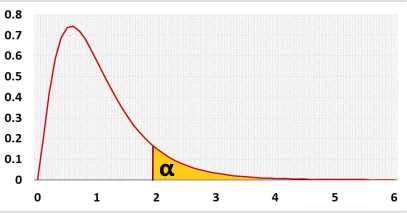
The F statistic represents a connection of the SSCP between the groups (H) and the SSCP within the groups (E) error. Unlike many other statistic tests, the smaller the F statistic the more likely the averages are equal.

F distribution
As with ANOVA, we compare between-groups to within-groups using the F distribution, but instead of using only the Sum of Squares (variances), we use both Sum of Squares and Cross Products (variances and covariances of dependent variables).
A similar result can be obtained by one of the following statistics: Wilks' Lambda, Pillai’s trace, Hotelling-Lawley trace, Roy’s maximum root.
Each statistic examines the variance in data in a different way depending on how it combines the dependent variables
In general, Wilks' lambda is the most commonly used statistic due to its simplicity, but we recommend to use the Pillai's trace. The Pillai's trace offers the greatest protection against Type I errors, it is a bit more powerful and more more robust against violations of the homogeneity assumption for covariance matrices.
p - number of dependent variables [Y1, Y1, . , Yp], number of columns.
g - number of groups/treatments, number of rows.
n - number of subjects, number of observations for one dependent variable (Yi), the number of values in one column.
λi - eigen value i.
We use the noncentral F distribution for the alternative assumption (h1). The non central parameter is: Wilks' Lambda:
ncp = f 2 *n*b
Pillai’s trace and Hotelling-Lawley trace:
ncp = f 2 *n*s
Currently for Roy's maximum root statistic we calculate the power of Pillai’s trace.
Calculate for each subject:
D 2 =(Yi-Ȳ) T S -1 (Yi-Ȳ)Y-the dependent variable vector for one subject.
Ȳ - average vector, contain the averages of each column.
Yi-Ȳ: one row in the DTotal matrix.
df = p. (number of dependent variables)
Sample data from all compared groups
Calculate average of each cell, and each column (Yi). To calculate the average of a column use the data in all the cells in this column.
Calculate the Square and Cross Products matrix (SSCP) for each group.
1. Calculate the differences matrix (D), by subtracting the relevant group's average from each observation.
2. Calculate the Sum of Square and Cross Products matrix (SSCP) using the following matrix form formula:
Similarly to the SSCP groups calculation but in this case use the entire columns.
Calculate the Square and Cross Products matrix (SSCP) for the all the groups togather.
1. Calculate the differences matrix (D), by subtracting the total's average from each observation.
2. Calculate the Sum of Square and Cross Products matrix (SSCP) using the following matrix form formula: